FFT Analysis of an EFT/Burst Pulse Train

What's in an EFT burst?

IEC 61000-4-4 defines the EFT/Burst test: trains of fast transients coupled into power and signal lines. Each individual pulse has a rise time of 5 ns and a duration of 50 ns. The interesting part is what happens when you repeat that pulse thousands of times in a burst.

IEC 61000-4-4 itself defines both repetition rates, but doesn't prescribe which one to use — that's up to the product standard. Some product standards only require 5 kHz, others call for 100 kHz as well. What does the frequency spectrum look like for each? An FFT of the full burst train answers that question.

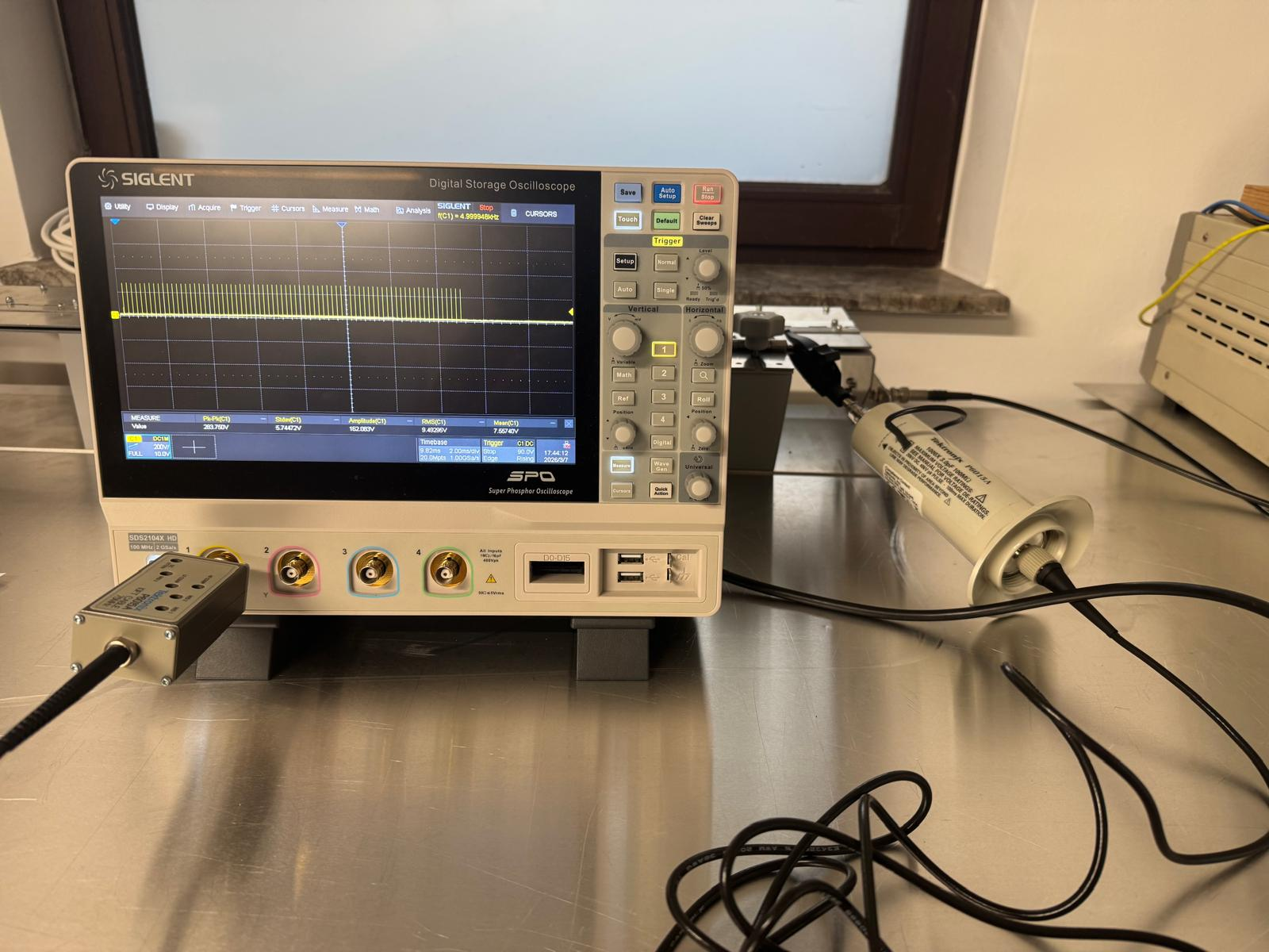
Equipment

• EFT/Burst generator for the pulse train at the specified voltage level and repetition rate
• Siglent SDS2104X HD oscilloscope — 12-bit ADC, 2 GSa/s, used for high-resolution waveform capture
• Tektronix P6015A high-voltage probe
• Python + SCPI — custom script to pull the full waveform (millions of samples) off the scope via Ethernet
• LTspice — PWL source driven by the captured waveform, used for FFT computation

Capturing the waveform

The scope was set to capture an entire burst — 75 pulses at both 5 kHz and 100 kHz repetition rates. At 2 GSa/s, that's tens of millions of samples per capture. A Python script connects to the scope via SCPI over TCP, downloads the raw 16-bit ADC data in chunks, converts it to voltage, and saves it as a NumPy archive.

The captured data is then converted into a PWL (piecewise linear) file that LTspice can use as a voltage source. Quiet regions between pulses are decimated to keep the file manageable while preserving full resolution around each pulse.

The single pulse

Before looking at the burst train, it's worth examining one individual pulse. The captured waveform shows the characteristic EFT shape: a fast rising edge (~5 ns rise time) followed by an exponential decay with a 50 ns time constant.

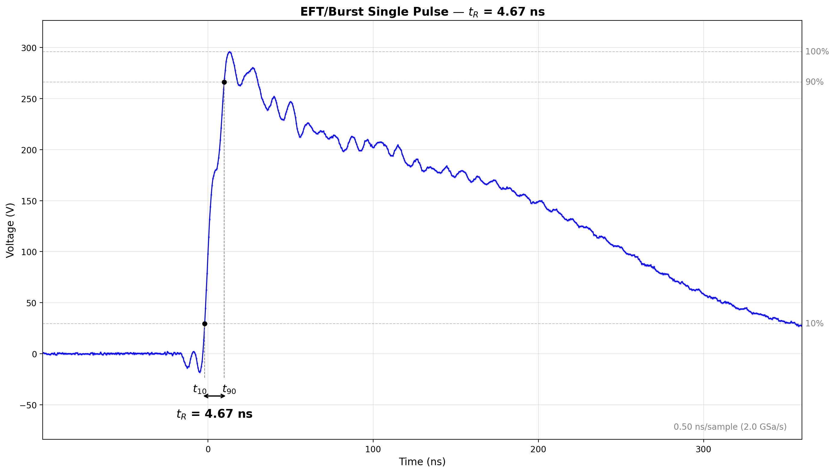
The measured rise time of 4.67 ns is in the same ballpark as the 5 ns IEC pulse, but this should be treated as an indicative capture, not a standards-grade verification. The P6015A probe is fast enough to show the pulse shape, but not ideal for claiming an accurate 5 ns rise-time measurement.

A note on the measurement: the standard defines the pulse shape into a 50 Ω load (t_r = 5 ± 1.5 ns, t_w = 50 ± 15 ns) and a 1000 Ω load (t_r = 5 ± 1.5 ns, t_w = 50 ns with -15/+100 ns tolerance). I captured the pulse directly at the capacitive coupling clamp, which presents neither load — the generator only sees the clamp's stray capacitance. So the waveform is not a standards-compliant verification measurement. That said, this is the actual voltage that gets induced into the clamp and coupled onto the cable, which is what matters for understanding the spectral content of the disturbance in practice.

The ringing after the peak is real — it comes from impedance mismatches in the generator output and coupling path.

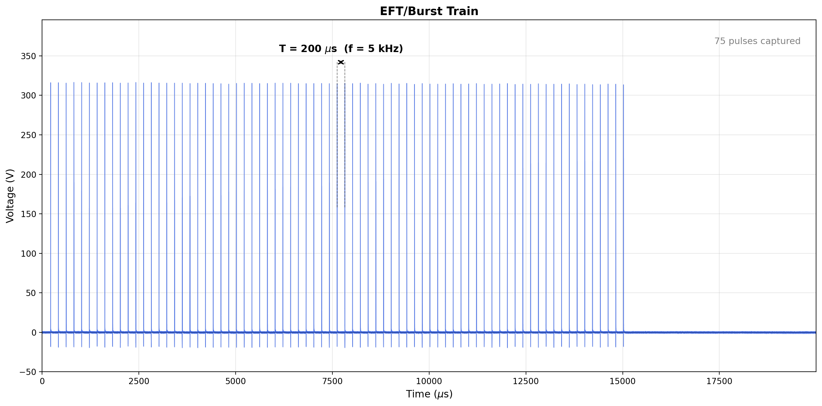
5 kHz burst train

At the standard 5 kHz repetition rate, pulses are spaced 200 µs apart. The burst lasts about 15 ms (75 pulses).

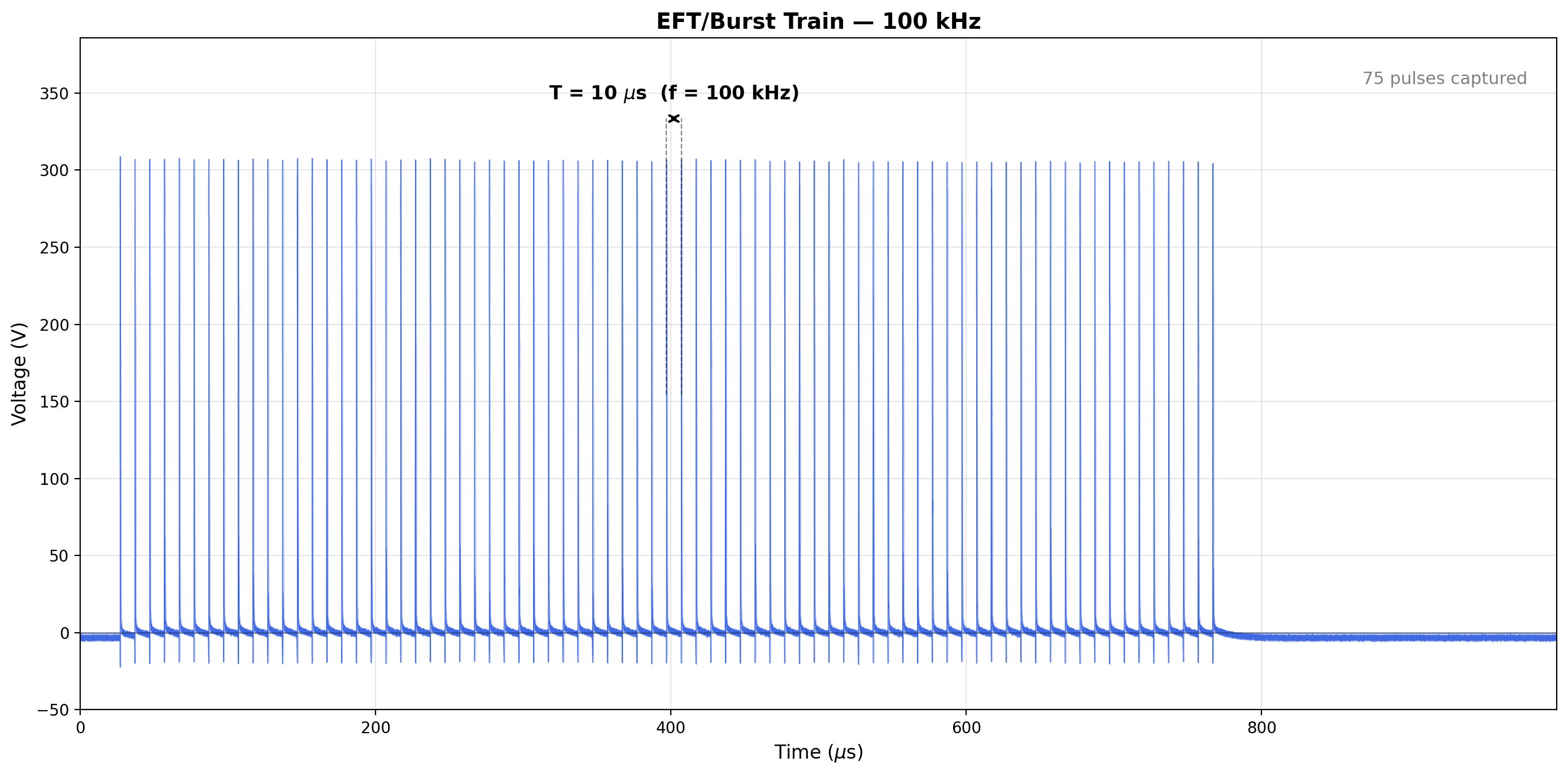
100 kHz burst train

At 100 kHz, pulses are only 10 µs apart — 20 times closer. The entire burst fits into less than 1 ms.

FFT: 5 kHz repetition rate

The captured waveform was fed into LTspice as a PWL source and the FFT was computed there. At 5 kHz repetition, the spectrum shows harmonics spaced at 5 kHz intervals. The envelope is relatively flat up to a few hundred kHz, then rolls off.

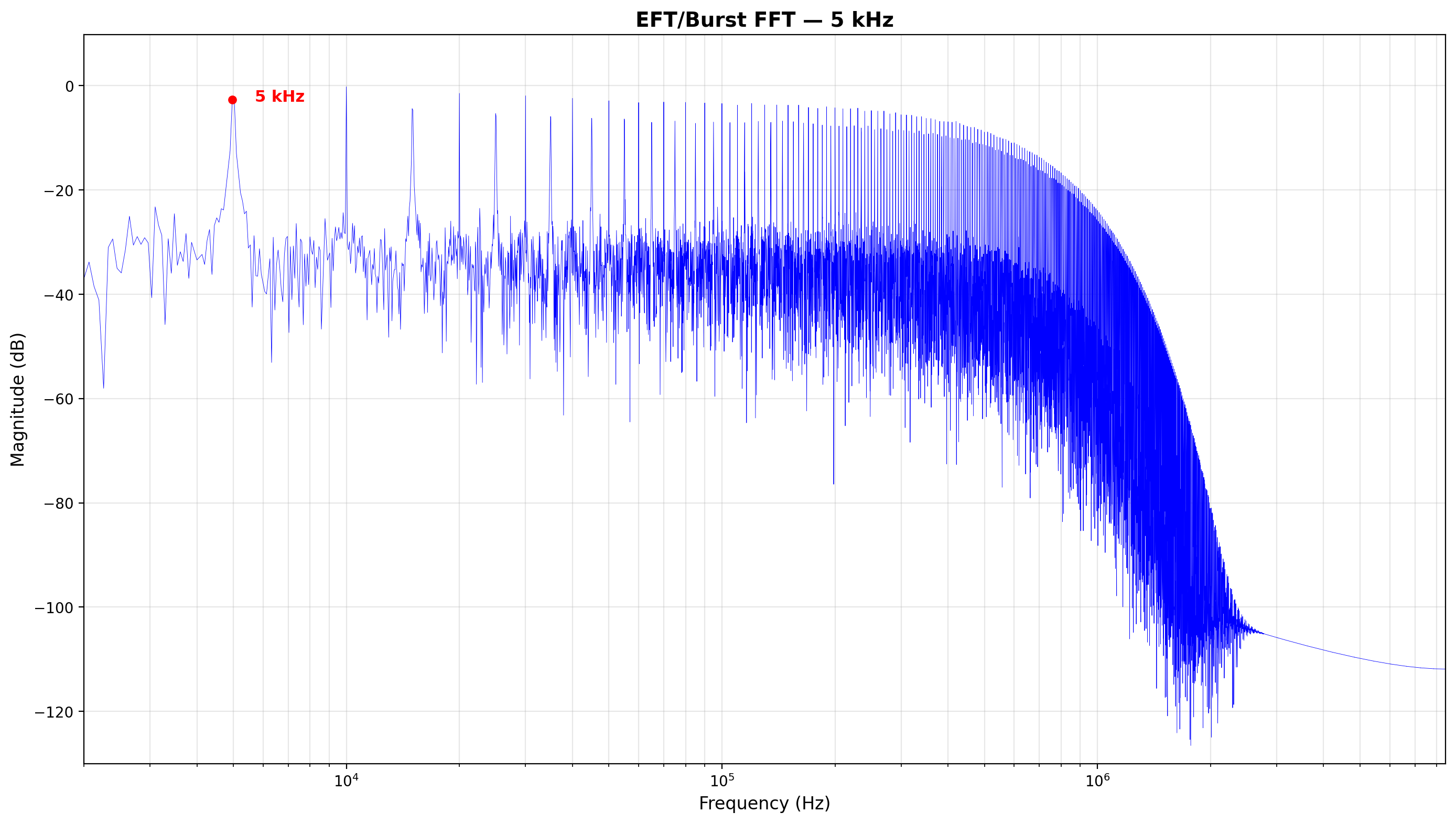
The spectral lines are dense because the 5 kHz spacing means there are many harmonics packed into each decade. The energy is spread across a wide range, but the peak levels are modest.

FFT: 100 kHz repetition rate

At 100 kHz, the harmonics are spaced 20 times further apart, so the individual lines are easier to distinguish. The high-frequency envelope is still set mainly by the pulse shape itself, not by the repetition rate.

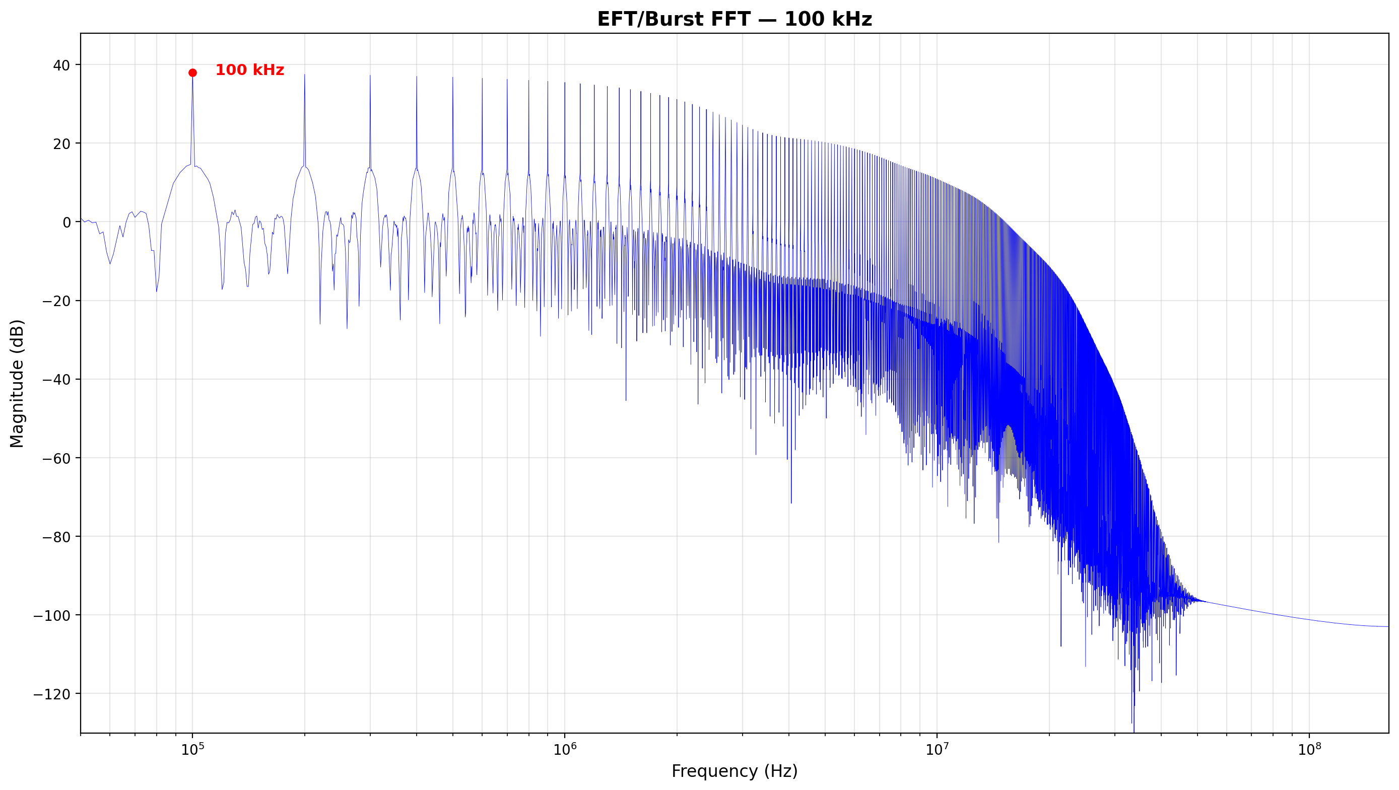
Note that the absolute dB levels between the two FFT plots should not be compared directly — the simulations used different time bases and normalization. What matters here is the comb structure: at 100 kHz, the line spacing is wider, while the overall high-frequency roll-off still comes from the pulse waveform and edge speed.

Why this matters for EMC

The 100 kHz test level exists because real switching transients repeat much faster than 5 kHz. A filter that handles the 5 kHz burst just fine might fail at 100 kHz.

Not all product standards require testing at both repetition rates. Some only specify 5 kHz, while others require 100 kHz as well. Check your applicable product standard to know which levels you actually need to pass.

Method

The full workflow:

1. Capture the burst train from a real generator using a scope at high sample rate (2 GSa/s)
2. Export the waveform as a PWL file for LTspice
3. Simulate in LTspice using the captured waveform as a voltage source
4. Compute the FFT in LTspice and export the frequency-domain data
5. Plot with Python (matplotlib) for fully customizable figures

LTspice gives you consistent windowing, which you don't easily get from the raw scope data. More importantly, once the captured waveform is in LTspice as a PWL source, you can place filter circuits, CDNs, or protection networks in front of it and simulate how they respond to a real burst.

All capture and plotting scripts are written in Python, using SCPI over TCP to control the oscilloscope.

Download the captured waveforms

The PWL files below contain the real captured burst waveforms, ready to use as voltage sources in LTspice. Drop them into your simulation and test your filter designs against a real EFT burst.

• 5 kHz burst train (PWL) — 85k data points, ~20 ms capture
• 100 kHz burst train (PWL) — 80k data points, ~1 ms capture