Before the Poor Man's Scanner Gets Retired

One more before it goes

I was about to put the Snapmaker away. The ground plane split scans were done and the 3D printer deserved to go back to being a 3D printer. But there was one more experiment I wanted to try.

About 10 years ago I watched Keith Armstrong's EMC presentations, and one demonstration stuck with me: a simple wire over a ground plane with a 90° bend. It's the most basic structure you can build, and it shows something fundamental about how return currents actually work. I repeated the experiment back then and it opened my eyes to EMC-ing (get it? EM-seeing). At that point I was struggling with my own boards failing, and this was the demo that made my return currents click. Min Zhang covers the same concept and explains the theory as well. Armstrong's series goes deeper into the practical implications.

At low frequencies, return current takes the path of least resistance. At higher frequencies, it takes the path of least inductance, which means it flows directly under the signal wire. When the wire makes a 90° turn, the return current has to negotiate that corner. How it does that depends on frequency. My scan covers 20 Hz to 100 kHz, which is where the transition from resistive to inductive return path behavior should happen on a board this size.

Test board

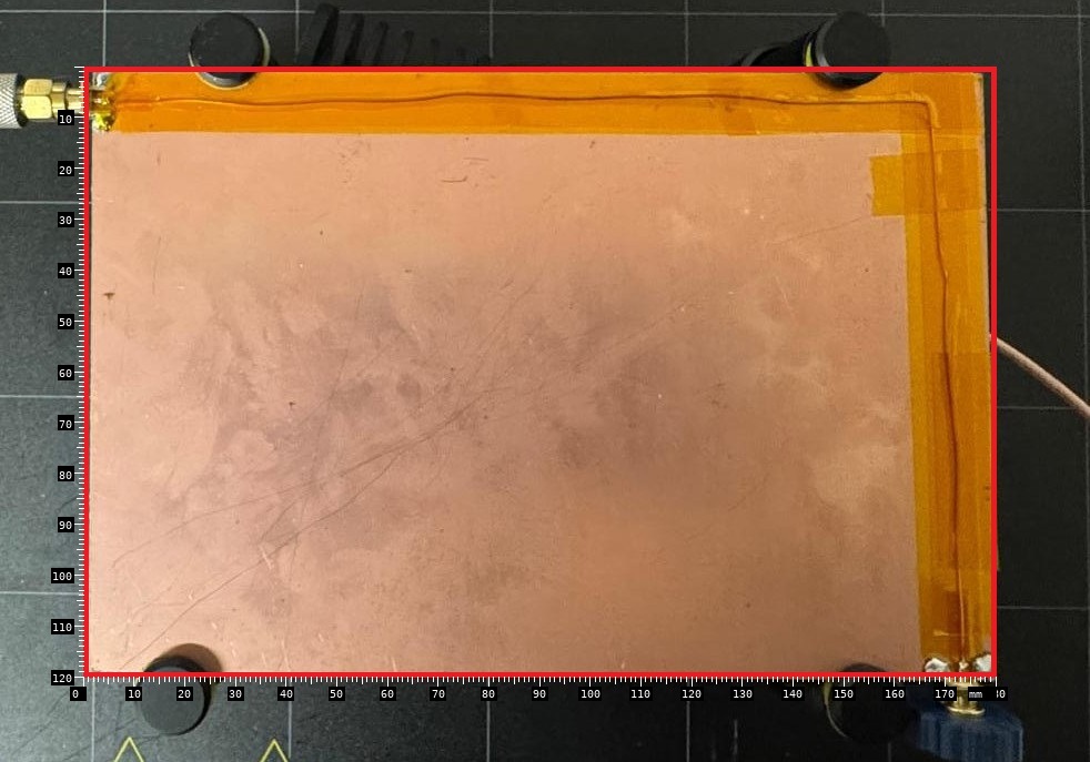
The test board consists of a 180 × 120 mm copper clad with a 90 degree wire running across 2 edges. I soldered 2 SMA connectors and terminated it with 50 Ω. I used kapton tape as 'prepreg'.

The setup is crude. The wire isn't perfectly straight, the solder joints aren't pretty, and the board has fingerprints all over it. But it should be good enough to demonstrate the principle. The red rectangle marks the scan area. I drew it in MS Paint because it makes it easy to align the photo with the 3D visualization, and I wasn't in the mood to figure out edge detection algorithms.

The problem

This is not a measurement you can do with standard near-field equipment. The Tekbox H-field probes I used in the previous articles are specified from 30 MHz upwards. They are passive loops, and their sensitivity rolls off hard below a few MHz. Same story with the spectrum analyzer: the Siglent SSA3032X-R starts at 9 kHz in principle, but it is not a tool designed for audio-frequency magnetic field measurements.

I wanted to use the same approach as before: feed a harmonic comb into the board, scan with a probe on the 3D printer, capture the full spectrum at each grid point. But there is no off-the-shelf comb generator that produces harmonics at 10 or 20 Hz. And no spectrum analyzer in my lab covers 20 Hz to 100 kHz with the resolution and dynamic range needed for this kind of spatial scan.

I was stuck for a while.

The equipment nobody thinks of

Then I remembered what was sitting on the shelf behind me.

A Stanford Research Systems SR780 Dynamic Signal Analyzer. Two-channel, DC to 102.4 kHz, 90 dB dynamic range, 800-line FFT. This is a 1990s instrument designed for vibration analysis and acoustic measurements, not EMC. But it does exactly what I need: high-resolution spectral analysis from near-DC to 100 kHz. It even has a built-in source output for driving the board.

That solved the analyzer problem. But how do you sense current at 20 Hz with spatial resolution?

The answer was also on the shelf: an Aim-TTi IProber 520. This is not a regular current probe. It uses a fluxgate magnetometer, a technology older than I am. Instead of relying on electromagnetic induction (which needs a changing field, meaning it gets worse at low frequencies), the fluxgate directly measures the static magnetic field. It works from DC. You place it near a conductor and it tells you how much current flows underneath, regardless of frequency.

Dave Jones explains the fluxgate principle in this video.

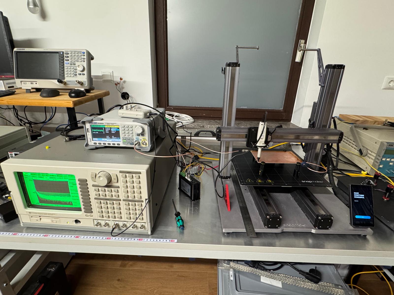
The IProber is a positional probe: it does not clamp around a wire. You hold it close to the surface and it measures the field at that point. That makes it perfect for scanning on a grid, exactly like the near-field probes from the previous articles. I 3D-printed a holder to mount it on the Snapmaker toolhead.

Building the signal source

There is no commercial comb generator for 20 Hz. So I built one.

A harmonic comb is mathematically simple. You sum sinusoids at integer multiples of a fundamental frequency:

$$x(t) = \sum_{n=1}^{N} \sin(2\pi \cdot n \cdot f_0 \cdot t + \varphi_n)$$

where $f_0$ is the fundamental, $N$ is the number of harmonics you want to have, and $\varphi_n$ are the phases. If you set all phases to zero, the peaks add up constructively and the crest factor is terrible. Randomizing the phases spreads the energy more evenly in time and brings the crest factor down from ~√N to roughly 3-4. The spectrum stays flat.

I computed the waveform in Python, converted it to a 16-bit binary file, and uploaded it to a Siglent SDG6052X arbitrary waveform generator over TCP. One waveform period, played in a loop, produces a continuous comb that is flat across the entire frequency range.

Getting the IProber to actually see the comb took more effort than I expected. The SDG output into a 50 ohm terminated board does not produce much current, and the IProber needs a decent signal to show anything above the noise floor. I spent a while staring at a flat spectrum wondering what was wrong. In the end I had to amplify the source to push more current through the board. Once there was enough current flowing, the comb harmonics appeared on the SR780 screen and the measurement became usable.

The scan needed two passes with different comb settings:

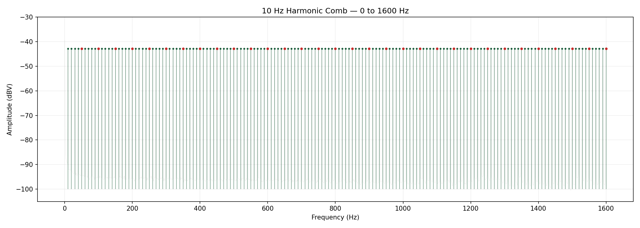
• 10 Hz fundamental, harmonics up to 1.6 kHz: 160 comb lines at 10 Hz spacing. The SR780 was set to 0-1600 Hz span with 800 lines (2 Hz/bin). Each 10 Hz harmonic lands exactly on a bin.

• 1024 Hz fundamental, harmonics up to 102.4 kHz: 100 comb lines. The SR780 was set to 0-102.4 kHz span with 800 lines (128 Hz/bin). The comb frequency has to be a multiple of the bin width, otherwise the peaks fall between bins and you lose amplitude. 1024 Hz = 8 × 128 Hz.

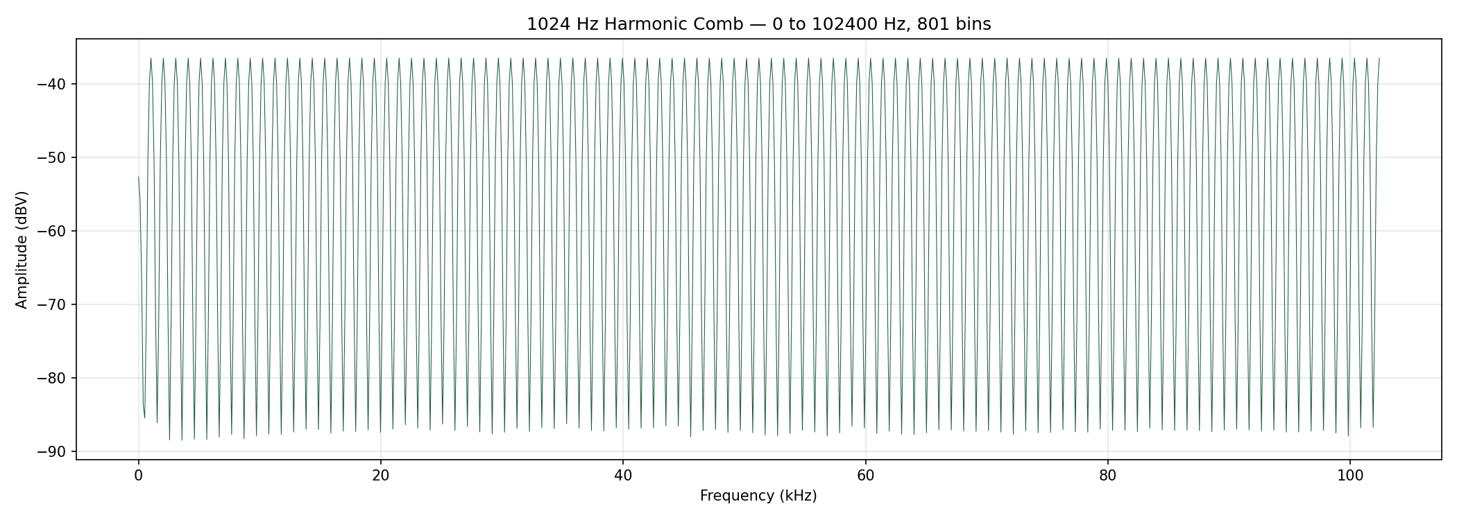
Getting the comb to land exactly on the FFT bins took some iteration. If the frequencies do not align, the spectral leakage smears the peaks and the spatial contrast drops.

Running the scan

Each scan takes about 1 hour 45 minutes. 925 grid points at 5 mm spacing, 180 × 120 mm area. At each point: move the gantry, wait 2 seconds for the FFT to settle, pull 801 data points over RS-232 at 19200 baud, save to disk, move to the next point. The SR780 talks RS-232 because that is what it has. No Ethernet, no USB, no GPIB on my setup. Reading 801 ASCII floats over a serial port is not fast. Each scan produces 925 × 801 = 740,925 data points, and there are four scans.

Each board orientation (probe in X, probe in Y) is a separate scan. Two orientations per comb setting, two comb settings: four scans total, roughly 7 hours of scanning. That is 2,963,700 data points pulled one by one over a serial port from a 1990s instrument. #OldiesButGoldies

The 50 Hz mains and its harmonics show up everywhere because the setup is not shielded. I captured an ambient trace with the comb turned off and subtracted it from the scan data. The probe's frequency response was also compensated: the comb should be flat, so any slope in the measured comb is the probe response. I computed correction factors to flatten it and applied them to all grid points.

The two probe orientations are combined as $\sqrt{H_x^2 + H_y^2}$ to get the total field magnitude at each point.

Results

Drag to rotate, scroll to zoom, right-drag to pan. Use the slider to step through frequencies from 20 Hz to 100 kHz. The board photo is overlaid on the terrain at the bottom.

At the lowest frequencies, the field is spread across the entire board. There is no clear concentration under the wire. Around 3.1 kHz the field starts to pull toward the trace. Above 30 kHz most of it is along the wire.

This is the transition from resistive to inductive return path behavior, measured spatially on a real board.

If you look closely at the ridge at higher frequencies, it follows the slight wiggliness of the wire. The wire is not perfectly straight on the board, and the current path tracks every bend. The scanner resolves this at 5 mm grid spacing.

There is something satisfying about pulling data from an instrument that was built before the web existed and rendering it as an interactive 3D terrain in a browser. The SR780 does not know what WebGL is. It does not need to. It just measures, reliably, one FFT at a time, the same way it has for almost 40 years. The visualization is new. The physics and the instrument are not. Sometimes the best tool for the job is the one that has been sitting on the shelf the longest.